Elastic Born modeling in an ocean-bottom node acquisition scenario

Introduction

In four-component ocean-bottom node (OBN) acquisition, the pressure wave is recorded by a hydrophone suspended in the water layer just above the sea floor. Additionally, three-component geophones are attached to the sea floor and record the vertical and two perpendicular horizontal particle velocities. The source is an airgun fired at the water surface. The upgoing wave can be distinguished from the downgoing wave by comparing the vertical geophone data to the hydrophone data. Whereas in the hydrophone data both the downgoing and the upgoing wave will have a positive polarity (assuming positive reflection coefficients in the subsurface), the value of the geophone data depends on the wave's vertical propagation direction. The downgoing wave will register on the vertical geophone with a negative polarity, while the upgoing wave will have a positive polarity.

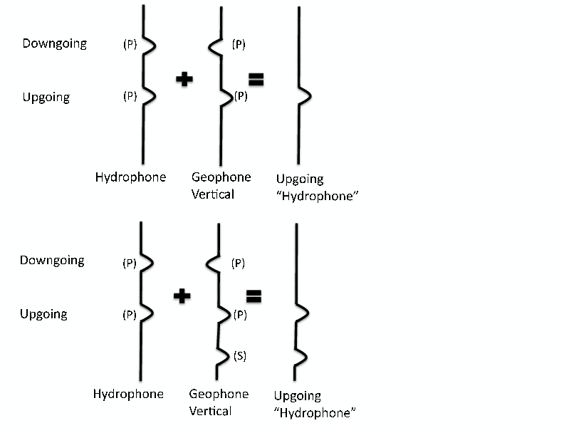
This characteristic has led to the PZ summation methodology (Barr and Sanders, 1989). With a proper scaling factor, the sum of the hydrophone and the vertical geophone should result in the upgoing waves only, while their difference should yield the downgoing wave only. This differentiation between the energy propagation direction at the sea floor has several applications. One of these applications is the ability to create separate images of the upgoing waves and of the downgoing waves that are reflected off the water surface, also known as the ``mirror-image'' (Ronen et al., 2005; Wong et al., 2009).

The PZ summation methodology, however, assumes that the energy recorded in the hydrophone and in the vertical geophone is mostly pressure wave energy. For the hydrophone, since it is within the water column, this assumption holds. However, if significant amounts of other wave modes are recorded by the geophone, then the PZ summation will not handle them properly, and will in effect introduce them into either the upgoing or the downgoing field. The sketch in Figure 1 displays this issue for the case where PZ summation is used to extract the upgoing data. Later processing steps (such as mirror-imaging), which rely on the assumption that the separated upgoing or downgoing data contains only acoustic arrivals, may have their results affected in turn.

up-down-sketch Figure 1. Simplified sketch of PZ summation. Top: For acoustic data, the summation of the hydrophone data and the vertical geophone data will result in the downgoing energy being eliminated, leaving only upgoing pressure data. Bottom: If the data contains shear waves, they will be recorded only by the geophone, and the PZ summation will mistakingly insert them into the result as upgoing pressure data.

In this paper I show the effect of imperfect PZ summation, as a result of significant shear wave energy existing in the vertical geophone, on the imaging of the upgoing wavefield.

In order to create single-scattered OBN synthetic data and run RTM with such data as input, I formulated and coded an elastic Born modeler. The special case of OBN acquisition necessitated a special manipulation of the smooth and the perturbed velocity models required to carry out Born modeling. The geophone receiver data was synthesized by recording the particle velocities of the single-scattered wavefield at the sea bed, and the hydrophone data was synthesized by recording the average of the normal stresses just above the sea bed, in the water-column.

The elastic propagation code is two dimensional, and all following examples are 2D as well. The gridding method I used for the elastic propagation was the Virieux staggered grid (Virieux, 1986), in which some wavefield values are located at grid points, and some are located at half-grid points, both spatially and temporally. The actual values which are propagated are the normal and transverse stresses $\left( \sigma_{xx}, \sigma_{zz}, \sigma_{xz} \right)$ , and the vertical and horizontal particle velocities $\left( v_x, v_z \right)$ . The P and S wavefields are extracted from the particle velocity fields by applying either the divergence or the curl operator to them, respectively.

For imaging of the P and S-wave modes in the elastic source and receiver wavefields, I follow the vector potential imaging condition discussed in Yan and Sava (2008). As they mention, the imaging results for full elastic propagation suffer from spurious modes being created when particle velocity data are injected as a boundary condition into the receiver wavefield during elastic RTM. In other words, injection of recorded P-wave particle velocities in an elastic medium will invariably create a P-wave and an S-wave mode. These injected spurious modes will, at the imaging stage, give rise to artifacts. This problem is similar to the problem of multiple generation in the receiver wavefield when a non-smooth model is used.

There are more advanced methods for achieving both up/down separation in conjunction with P/S separation, in the data domain. Dankbaar (1985), Wapenaar et al. (1990), Amundsen (1993) and Schalkwijk et al. (2003) have all shown methods which can separate pressure and shear waves in the data, as well as separating upgoing from downgoing. However these methods require good knowledge of medium parameters at the sea bed where the geophones are located. Furthermore, it is not correct to assume that the data are composed of pressure and shear body waves only. In OBN acquisition (as in land acquisition) surface waves can contaminate the data.

Elastic Born modeling in an ocean-bottom node acquisition scenario