 |
 |
 |
 | Least-squares wave-equation inversion of time-lapse seismic data sets - A Valhall case study |  |
![[pdf]](icons/pdf.png) |
Next: Case study
Up: Ayeni and Biondi: Valhall
Previous: Introduction
Given a linearized modeling operator  , the seismic data
  for survey
  due to a reflectivity model
  is
is
 |
(1) |
Assuming we have two data sets (baseline
 and monitor
 ) acquired at different times over an evolving reservoir, joint least-squares migration/inversion involves solving the following regression:
![\begin{displaymath}\begin{array}{ccc} \left [ \begin{array}{cc} {\bf L}_{0} & {\...
...0} \\ {\bf0} \\ \hline {\bf0} \end{array} \right ] \end{array},\end{displaymath}](img10.png) |
(2) |
where
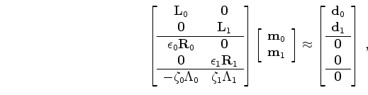 and
and
 are the spatial and temporal regularization operators respectively, and
 and
and
 are the corresponding regularization parameters.
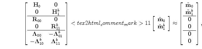
Although we can directly solve equation 2 by minimizing the quadratic-norm of the regression (Ajo-Franklin et al., 2005), we choose to transform it to an image space problem of the form (Ayeni and Biondi, 2011)
are the corresponding regularization parameters.
Although we can directly solve equation 2 by minimizing the quadratic-norm of the regression (Ajo-Franklin et al., 2005), we choose to transform it to an image space problem of the form (Ayeni and Biondi, 2011)
![\begin{displaymath}\begin{array}{c} \left [ \begin{array}{ccc} {\bf H_0 } & {\bf...
...\\ \hline {\bf0} \\ {\bf0} \\ \end{array} \right ], \end{array}\end{displaymath}](img15.png) |
(3) |
where
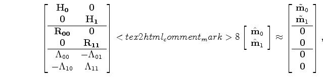 is the wave-equation Hessian, and
 and
and
 are the spatial and temporal constraints.
The inverted time-lapse image
are the spatial and temporal constraints.
The inverted time-lapse image
 is then the difference between the inverted baseline and monitor images (
 and
and
 ).
Equation 3 can be extended to multiple seismic data sets (Ayeni and Biondi, 2010).
Alternatively, we can re-write equation 3 to invert directly for the time-lapse image and a static baseline image (Ayeni and Biondi, 2011).
Due to physical movements of reflectors and velocity changes (e.g., due to reservoir depletion and compaction) between surveys, the baseline and monitor images will not be aligned.
Such misalignments must be accounted for before or during inversion.
As is the case in many practical time-lapse monitoring problems, we assume that the monitor data are migrated with the baseline velocity, which has been estimated to a high accuracy.
However this method can be applied where an accurate monitor velocity has been available.
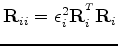
The updated inversion problem is then given by (Ayeni and Biondi, 2011)
).
Equation 3 can be extended to multiple seismic data sets (Ayeni and Biondi, 2010).
Alternatively, we can re-write equation 3 to invert directly for the time-lapse image and a static baseline image (Ayeni and Biondi, 2011).
Due to physical movements of reflectors and velocity changes (e.g., due to reservoir depletion and compaction) between surveys, the baseline and monitor images will not be aligned.
Such misalignments must be accounted for before or during inversion.
As is the case in many practical time-lapse monitoring problems, we assume that the monitor data are migrated with the baseline velocity, which has been estimated to a high accuracy.
However this method can be applied where an accurate monitor velocity has been available.
The updated inversion problem is then given by (Ayeni and Biondi, 2011)
![\begin{displaymath}\begin{array}{c} \left [ \begin{array}{ccc} {\bf H }_{0} & {\...
...\\ \hline {\bf0} \\ {\bf0} \\ \end{array} \right ], \end{array}\end{displaymath}](img22.png) |
(4) |
where
 and
and
 are respectively the migrated and inverted monitor images repositioned (warped) to the baseline image.
The superscript
are respectively the migrated and inverted monitor images repositioned (warped) to the baseline image.
The superscript  on the operators denotes that they are referenced to the baseline image.
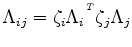
For example,
on the operators denotes that they are referenced to the baseline image.
For example,
 is the Hessian computed with the monitor geometry but with the baseline velocity.
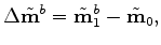
Note that the conventional time-lapse image
is the Hessian computed with the monitor geometry but with the baseline velocity.
Note that the conventional time-lapse image
 estimated at the baseline position is given by
 |
(5) |
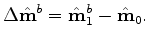
while the inverted time-lapse image
 is given by
 |
(6) |
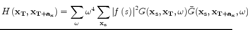
For any practical application, it is infeasible (and unnecessary) to compute the full Hessian matrix.
Because the problem is posed in the image space, we only need to compute the Hessian for a target region of interest around the reservoir.
In addition, we only compute off-diagonal elements sufficient to capture the dominant structure of the Hessian.
This target-oriented approximation of the Hessian is given by (Valenciano et al., 2006)
 |
|
|
|
 |
|
|
(7) |
where
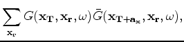 is an image point within the target area, and
 represents points within a small region around
.
For any image point, elements of
represents points within a small region around
.
For any image point, elements of
 represent a row of a sparse Hessian matrix
  whose non-zero components are defined by
 .
Therefore,
defines the number of off-diagonal elements of the Hessian that are computed -- which represents the size of the point spread function (PSF) at each image point (Lecomte and Gelius, 1998; Valenciano et al., 2006; Chavent and Plessix, 1999).
.
Therefore,
defines the number of off-diagonal elements of the Hessian that are computed -- which represents the size of the point spread function (PSF) at each image point (Lecomte and Gelius, 1998; Valenciano et al., 2006; Chavent and Plessix, 1999).
 is the complex conjugate of Green's function
  at frequency
  ;
;
 is the source function; and
 and
and
 are the source and receiver positions, respectively.
Note that because of symmetry, only one half of the approximate Hessian is required.
In this paper, we follow the phase-encoding approach of Tang (2009) to efficiently compute the target-oriented Hessian.
The spatial regularization operators in equation 4 are non-stationary directional Laplacians (Hale, 2007), whereas the temporal constraint is the difference between the aligned images.
Further review of the methodology is given by Ayeni and Biondi (2011,2010)
are the source and receiver positions, respectively.
Note that because of symmetry, only one half of the approximate Hessian is required.
In this paper, we follow the phase-encoding approach of Tang (2009) to efficiently compute the target-oriented Hessian.
The spatial regularization operators in equation 4 are non-stationary directional Laplacians (Hale, 2007), whereas the temporal constraint is the difference between the aligned images.
Further review of the methodology is given by Ayeni and Biondi (2011,2010)
|
|
|
|
| Least-squares wave-equation inversion of time-lapse seismic data sets - A Valhall case study | |
|
Next: Case study
Up: Ayeni and Biondi: Valhall
Previous: Introduction
2011-09-13