Subsalt velocity analysis by target-oriented wavefield tomography: A 3-D field-data example

Migrating the original data set using the updated velocity model

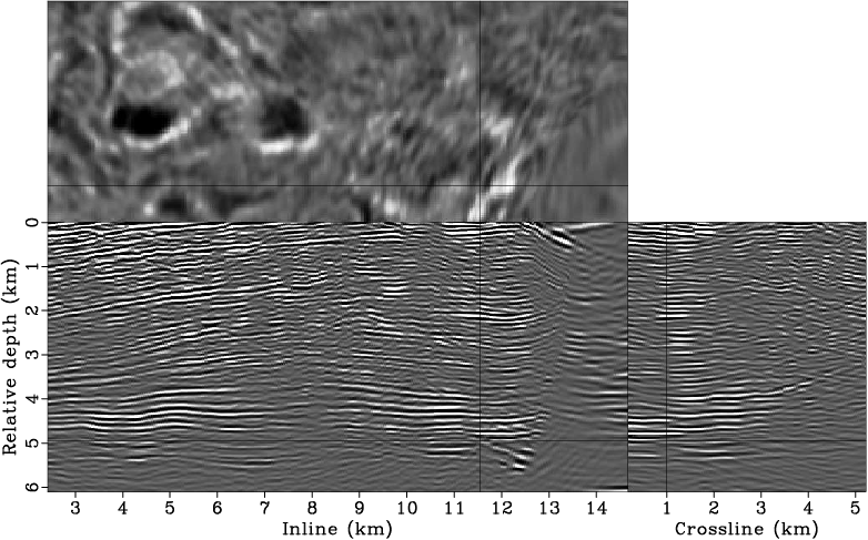
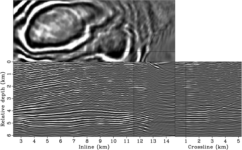
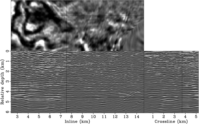
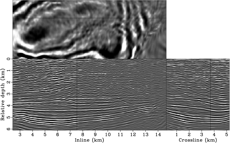
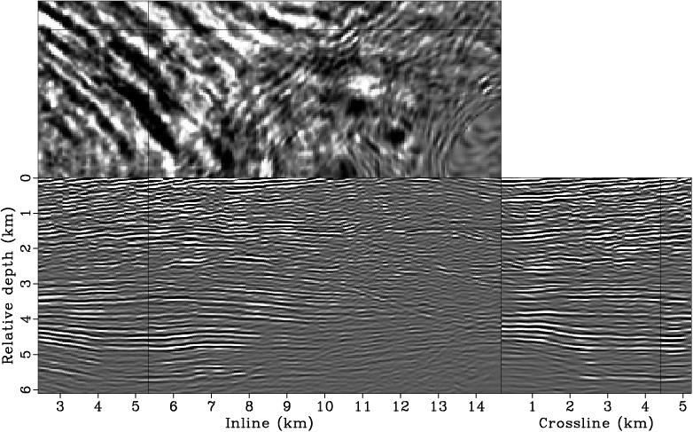
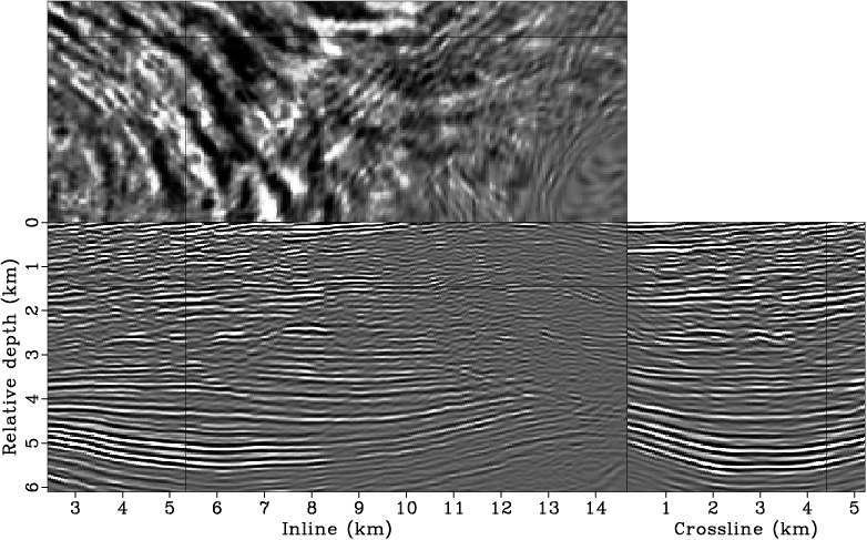
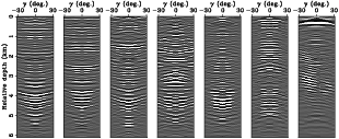
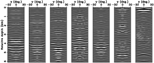
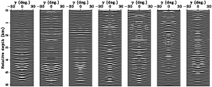
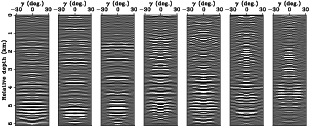
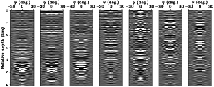
After the tomographic inversion step, we migrate the original data set using the updated velocity model. Once again, we perform 3-D conical wave migration and normalize the migrated image with the diagonal of the phase-encoded Hessian, also computed using the updated velocity model, to compensate for uneven subsurface illumination. The updated image (Figures 11(b), 12(b) and 13(b)) significantly improves the continuity of the reflectors in both the inline and crossline directions and is also more focused than the initial one (Figures 11(a), 12(a) and 13(a)). Figures 14, 15 and 16 show the corresponding angle-domain common-image gathers (ADCIGs) before and after updating the velocity model. The flatness and coherence of ADCIGs have been improved considerably after updating the subsalt velocities.

bpgom3d-bimg-cpst1,bpgom3d-imag-cpst1
Figure 11. Comparison between the zero-subsurface-offset image (a) before and (b) after updating the velocities. Both results are obtained using the original surface-recorded data set. In both panels, the crosshair is taken at inline $11.55$ km, crossline $1.00$ km and relative depth $4.94$ km. [CR]

bpgom3d-bimg-cpst2,bpgom3d-imag-cpst2
Figure 12. Comparison between the zero-subsurface-offset image (a) before and (b) after updating the velocities. Both results are obtained using the original surface-recorded data set. In both panels, the crosshair is taken at inline $7.55$ km, crossline $3.70$ km and relative depth $4.57$ km. [CR]

bpgom3d-bimg-cpst3,bpgom3d-imag-cpst3
Figure 13. Comparison between the zero-subsurface-offset image (a) before and (b) after updating the velocities. Both results are obtained using the original surface-recorded data set. In both panels, the crosshair is taken as inline $5.35$ km, crossline $4.40$ km and relative depth $1.46$ km. [CR]

adcig2d-bvel-cpst1,adcig2d-invt-cpst1
Figure 14. Comparisons between ADCIGs (a) before and (b) after updating the velocities. Both results are obtained using the original surface-recorded data set. All of the ADCIGs are extracted at the same crossline ($1.00$ km), but at inlines $1.52$, $3.05$, $4.57$, $6.10$, $7.62$, $9.14$ and $10.67$ km, from left to right. [CR]

adcig2d-bvel-cpst2,adcig2d-invt-cpst2
Figure 15. Comparisons between ADCIGs (a) before and (b) after updating the velocities. Both results are obtained using the original surface-recorded data set. All of the ADCIGs are extracted at the same crossline ($3.70$ km), but at inlines $1.52$, $3.05$, $4.57$, $6.10$, $7.62$, $9.14$ and $10.67$ km, from left to right. [CR]

adcig2d-bvel-cpst3,adcig2d-invt-cpst3
Figure 16. Comparisons between ADCIGs (a) before and (b) after updating the velocities. Both results are obtained using the original surface recorded data set. All of the ADCIGs are extracted at the same crossline ($4.40$ km), but at inlines $1.52$, $3.05$, $4.57$, $6.10$, $7.62$, $9.14$ and $10.67$ km, from left to right. [CR]

Subsalt velocity analysis by target-oriented wavefield tomography: A 3-D field-data example