|
|
|
|
Subsalt velocity analysis by target-oriented wavefield tomography: A 3-D field-data example |
We perform conical-wave migration (Duquet et al., 2001; Whitmore, 1995; Liu et al., 2006; Zhang et al., 2005)
to generate the initial image gathers, where
we synthesize ![]() conical waves for each crossline and migrate
conical waves for each crossline and migrate ![]() conical waves in total.
The minimum and maximum inline take-off angles at the surface for the conical waves are
conical waves in total.
The minimum and maximum inline take-off angles at the surface for the conical waves are ![]() and
and ![]() , respectively.
The maximum frequency used for the initial migration is
, respectively.
The maximum frequency used for the initial migration is ![]() Hz.
We also compute the diagonal of the Hessian in the conical-wave domain using the phase-encoding method (Tang, 2009),
which encodes the source-side Green's functions using inline plane-wave phase-encoding functions and the receiver-side
Green's functions using random-phase encoding functions. The simultaneous encoding dramatically reduces the
computational cost of the Hessian (Tang and Biondi, 2011).
Hz.
We also compute the diagonal of the Hessian in the conical-wave domain using the phase-encoding method (Tang, 2009),
which encodes the source-side Green's functions using inline plane-wave phase-encoding functions and the receiver-side
Green's functions using random-phase encoding functions. The simultaneous encoding dramatically reduces the
computational cost of the Hessian (Tang and Biondi, 2011).
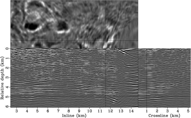
Figure 2 shows the zero-subsurface offset image
for the target region obtained using the initial velocity model (Figure 1).
The image has been normalized with the diagonal of the Hessian (not shown here).
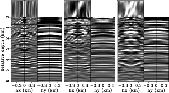
To more accurately preserve the velocity information, we compute both inline and crossline subsurface offsets
(Figure 3).
The crossline subsurface offset is included because
wavefields can travel out of plane during propagation, and therefore they may image the subsurface with different
azimuths than that on the surface.
The 3-D subsurface-offset-domain common-image gathers (SODCIGs) shown in
Figure 3 confirm this; the events in the top panels of Figures 3a
and 3b are tilted, suggesting that they are not imaged by zero subsurface azimuth.
Also note that the 3-D SODCIGs are not well focused at the zero subsurface offset in either the inline or crossline directions.
The defocusing in the inline subsurface offset (![]() ) is mainly caused by velocity inaccuracies, whereas the defocusing
in the crossline subsurface offset (
) is mainly caused by velocity inaccuracies, whereas the defocusing
in the crossline subsurface offset (![]() ) is mainly due to insufficient crossline data coverage
(single surface azimuth data)(Tang, 2007).
) is mainly due to insufficient crossline data coverage
(single surface azimuth data)(Tang, 2007).
|
|---|
|
bpgom3d-bimg-cpst1-copy
Figure 2. The zero-subsurface-offset-domain image migrated using the original data set and the initial velocity. The image has been normalized using the diagonal of the phase-encoded Hessian. [CR] |
|
|
|
|---|
|
bpgom3d-cig3d-orig-cpst
Figure 3. The Hessian-normalized 3-D SODCIGs obtained using the original data set and the initial velocity model. Panels (a), (b) and (c) are extracted at |
|
|
|
|
|
|
Subsalt velocity analysis by target-oriented wavefield tomography: A 3-D field-data example |