 |
 |
 |
 | Subsalt velocity analysis by target-oriented wavefield tomography: A 3-D field-data example |  |
![[pdf]](icons/pdf.png) |
Next: 3-D field-data examples
Up: Tang and Biondi: 3-D
Previous: introduction
We formulate our method under the framework of seismic data mapping (SDM) (Bleistein and Jaramillo, 2000; Hubral et al., 1996),
where the idea is to transform the original observed seismic data from one acquisition configuration to another with a designed
mapping operator. SDM can be summarized as two main steps:
(1) apply the (pseudo) inverse of the designed mapping operator to the original
data set to generate a model, and
(2) apply the forward mapping operator to the model to generate a new data set with a different
acquisition configuration than the original one.
In our case, we use generalized Born wavefield modeling to perform data mapping.
With an initial velocity model, seismic prestack images can be obtained using the pseudo-inverse of
the generalized Born modeling operator as follows:
 |
|
|
(1) |
where  and
and  denote adjoint and pseudo-inverse, respectively;
 is the seismic image;
 is the generalized Born modeling operator computed using an initial velocity model
  ,
whose adjoint
,
whose adjoint  is the well-known depth migration operator;
  is the Hessian
operator (Tang, 2009; Plessix and Mulder, 2004; Valenciano, 2008); and
is the Hessian
operator (Tang, 2009; Plessix and Mulder, 2004; Valenciano, 2008); and
 is the observed surface data.
It is important to note that the seismic image must be parameterized as a function
of both spatial location and some prestack parameter, such as the subsurface offset, reflection angle, etc.,
in order to preserve the velocity information for later velocity analysis (Tang and Biondi, 2010).
In this paper, we use the subsurface offset as our prestack parameter.
The significance of the Hessian operator in equation 1 is that
its pseudo-inverse removes the influence of the original acquisition
geometry in the least-squares sense, and the resulting image is independent from the original data.
However, the full Hessian is impossible to obtain in practice due to its size and computational cost;
we therefore approximate it by a diagonal matrix :
 .
We further reduce the cost of computing the diagonal of Hessian by using the phase encoding method (Tang, 2009; Tang and Lee, 2010; Tang, 2007).
.
We further reduce the cost of computing the diagonal of Hessian by using the phase encoding method (Tang, 2009; Tang and Lee, 2010; Tang, 2007).
We obtain a target image
 by applying a selecting operator
  to the initial image:
 ,
where the selecting operator can be simply a windowing operator.
A new data set
,
where the selecting operator can be simply a windowing operator.
A new data set
 can then be simulated as follows:
 |
|
|
(2) |
where
 is the Born modeling operator computed using
the same initial velocity , but with a different acquisition configuration.
The wavefield propagation can be restricted to regions with inaccurate velocities, and
the modeled data can be collected at the top of the target region. The target-oriented
modeling strategy makes the new data set much smaller than the original one.
The new data set can be imaged using the migration operator, i.e., the adjoint
of
is the Born modeling operator computed using
the same initial velocity , but with a different acquisition configuration.
The wavefield propagation can be restricted to regions with inaccurate velocities, and
the modeled data can be collected at the top of the target region. The target-oriented
modeling strategy makes the new data set much smaller than the original one.
The new data set can be imaged using the migration operator, i.e., the adjoint
of
 , with an arbitary velocity
  , as follows:
 |
|
|
(3) |
We pose the velocity estimation problem as an optimization problem
that seeks an optimum velocity model by minimizing a user-defined image residual
(or maximizing some measure of the image coherence). There are many ways of defining the objective
functions. In this paper, we use the differential semblance optimization (DSO) (Symes and Carazzone, 1991) as the
criterion to estimate the velocity. The DSO objective function in the subsurface-offset domain
is (Shen and Symes, 2008; Shen, 2004)
 |
|
|
(4) |
where
 is the image point in the subsurface and
 is the subsurface
offset.
The physical interpretation of the subsurface-offset-domain DSO is that it optimizes the velocity model
by penalizing energy at non-zero subsurface offset, taking advantage of the fact that
seismic events should focus at zero-subsurface offset if migrated using an accurate velocity model (Shen, 2004).
However, the gradient of the objective function defined by equation 4 is
sensitive to the amplitude variation of the images due to uneven illumination (Vyas and Tang, 2010; Fei and Williamson, 2010).
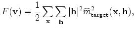
We propose to normalize the DSO objective function
by the square of the root-mean-squared (RMS) image amplitudes to reduce the influence of image amplitude variations.
The normalized DSO objective function is
is the subsurface
offset.
The physical interpretation of the subsurface-offset-domain DSO is that it optimizes the velocity model
by penalizing energy at non-zero subsurface offset, taking advantage of the fact that
seismic events should focus at zero-subsurface offset if migrated using an accurate velocity model (Shen, 2004).
However, the gradient of the objective function defined by equation 4 is
sensitive to the amplitude variation of the images due to uneven illumination (Vyas and Tang, 2010; Fei and Williamson, 2010).
We propose to normalize the DSO objective function
by the square of the root-mean-squared (RMS) image amplitudes to reduce the influence of image amplitude variations.
The normalized DSO objective function is
 |
|
|
(5) |
We use nonlinear conjugate-gradient method to minimize 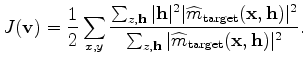 .
The gradient is calculated using the adjoint-state method
(with a one-way wave-equation formulation) without explicitly
computing the Jacobian matrix (Shen and Symes, 2008; Sava and Vlad, 2008; Tang et al., 2008).
.
The gradient is calculated using the adjoint-state method
(with a one-way wave-equation formulation) without explicitly
computing the Jacobian matrix (Shen and Symes, 2008; Sava and Vlad, 2008; Tang et al., 2008).
|
|
|
|
| Subsalt velocity analysis by target-oriented wavefield tomography: A 3-D field-data example | |
|
Next: 3-D field-data examples
Up: Tang and Biondi: 3-D
Previous: introduction
2011-05-24