Ambient seismic noise eikonal tomography for near-surface imaging at Valhall

Eikonal Tomography

Tomography produces an estimated velocity field from a large number of measurements of travel time (or phase). Traditionally, a forward-modeling operator is constructed by solving the eikonal equation in a background velocity model for each observable data point. These data points then act as a global constraint on the inversion. The resulting linear system is typically solved by matrix inversion techniques, regularized by spatial smoothing and Tichonov regularization. In contrast, eikonal tomography (Lin et al., 2009) is a procedure that uses the spatial gradient of a travel-time map as a local constraint on the wave-speed map. This relation is described by the scalar eikonal equation (Aki and Richards, 2002):

$$\left\vert \nabla t_i(x) \right\vert = c^{-1}_i(x).$$ (1)

Evaluating this equation for one virtual-source gather leads to an estimate of the local wave velocity.

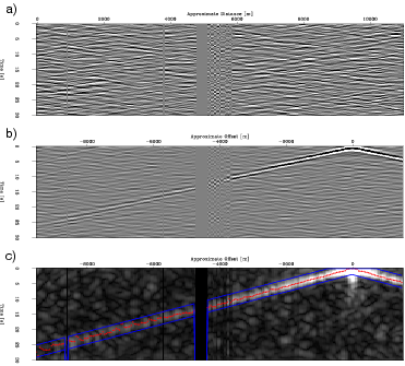
We perform ambient-seismic-noise eikonal tomography as follows: First, the data are bandpassed (for band C) and virtual-seismic source gathers are constructed by correlation. Figure 2a shows 30 seconds of bandpassed seismic noise recorded in the 2008 dataset by one line of the Valhall array. Figure 2b shows a virtual-source gather created by correlating 2 hours of noise along that line with the data for the station at the offset marked 0, located towards the right end of the line. For ideal ambient seismic noise, positive and negative time lags of the correlation should contain a symmetrized impulse response (Wapenaar and Fokkema, 2006). We stacked positive and negative time lags to enhance the quality of the created virtual-source gathers.

Next, traveltimes are estimated by picking the maximum value of the envelope function of the virtual-seismic-source data within a defined moveout window. Figure 2c shows picks for the virtual-source gather in figure 2b. We also calculate a signal-to-noise ratio (SNR) quality factor, defined as the amplitude of the envelope peak within the moveout window divided by the average amplitude outside the window. We keep only the traveltime picks exceeding a specified SNR and regularize them using biharmonic spline interpolation (Sandwell, 1987) (see Appendix ). The traveltime map should only be interpreted for portions surrounded by picks that we kept. Next, we use equation 1 to estimate the local velocity at each point for waves from each virtual-source gather. The final step is to produce tomographic maps by statistically characterizing the estimates at each position in the model.

$$s_0(x) = \frac{1}{N} \sum_{i=1}^N s_i(x)$$ (2)

and

$$\sigma_s^2(x) = \frac{1}{N(N-1)}\sum_i^N\left( s_i(x) - s_0(x) \right)^2.$$ (3)

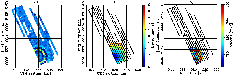
Figure 3 shows how this works. Figure 3a shows an amplitude snapshot for a virtual-source gather gather in the southern portion of the Valhall data for the 2008 dataset. Notice that the impulse response is nearly perfectly omnidirectional. Figure 3b shows regularized travel times across the array for this virtual-source. Note that more distant picks did not have a sufficient SNR and were discarded. Figure 3c shows a map of velocity estimates calculated using those regularized picked travel times. This process is repeated for each virtual-source gather, potentially producing a large number of velocity estimates.

Laura-V-picked
Figure 2. Three panels demonstrating the first half of the processing flow of ambient seismic noise eikonal tomography for a receiver line in the 2008 dataset: (a) 30 seconds of ambient seismic noise after bandpassing between 0.35 Hz and 1.75 Hz; (b) data from a virtual-source created at a station near the right end of the line; (c) travel-time picks superimposed on top of the envelope function of the virtual-seismic-source data in the middle panel.

Eikonal-tomo
Figure 3. Three panels showing the continuation of the processing flow begun in Figure 2, traveltime map construction and velocity estimation for one virtual-source: (a) A snapshot showing Scholte-waves propagating away from a virtual-source in the southern portion of the Valhall array. The virtual-source was created using data from the 2008 dataset, bandpassed between 0.35 Hz and 1.75 Hz. (b) Regularized travel time surfaces picked from this virtual-source gather. (c) The resulting velocity estimates.

Ambient seismic noise eikonal tomography for near-surface imaging at Valhall