|
|
|
|
An approximation of the inverse Ricker wavelet as an initial guess for bidirectional deconvolution |
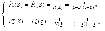
In the Z domain, the half-Ricker wavelet has two zeros, which makes it impossible to directly invert. Therefore, we modify the formula with two new factors to avoid errors caused by dividing by zero:
 and
and
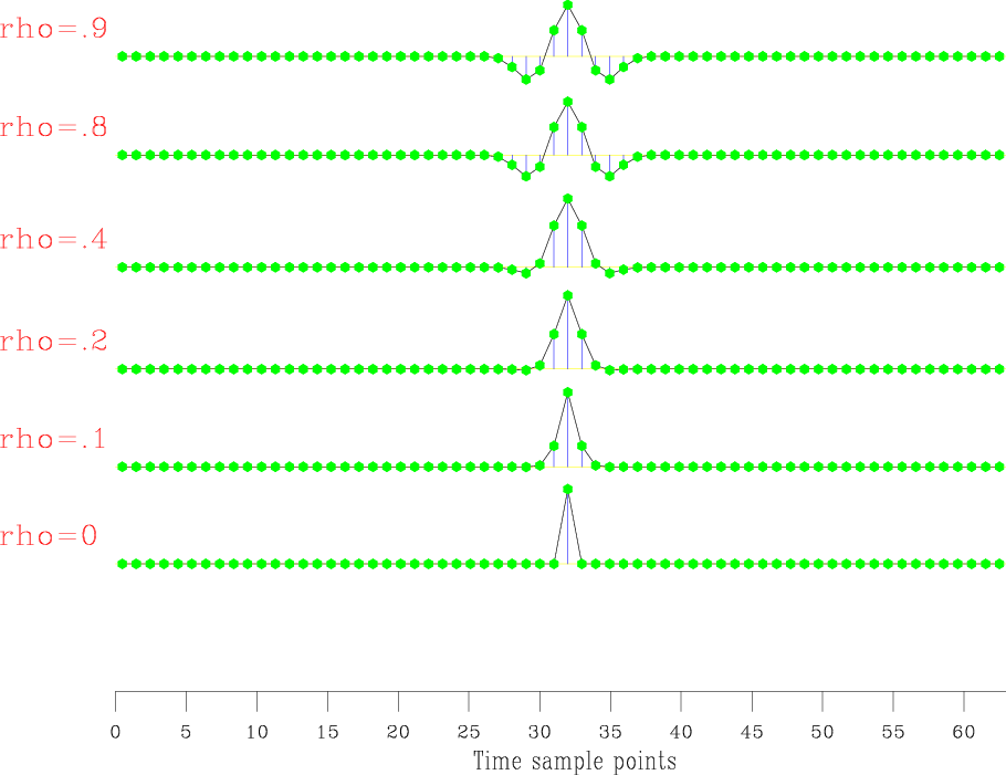
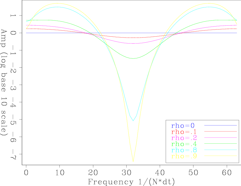
Figures 3(a) and 3(b) show the fourth-order Ricker wavelet in the time and frequency domains with different ![]() values.
values.
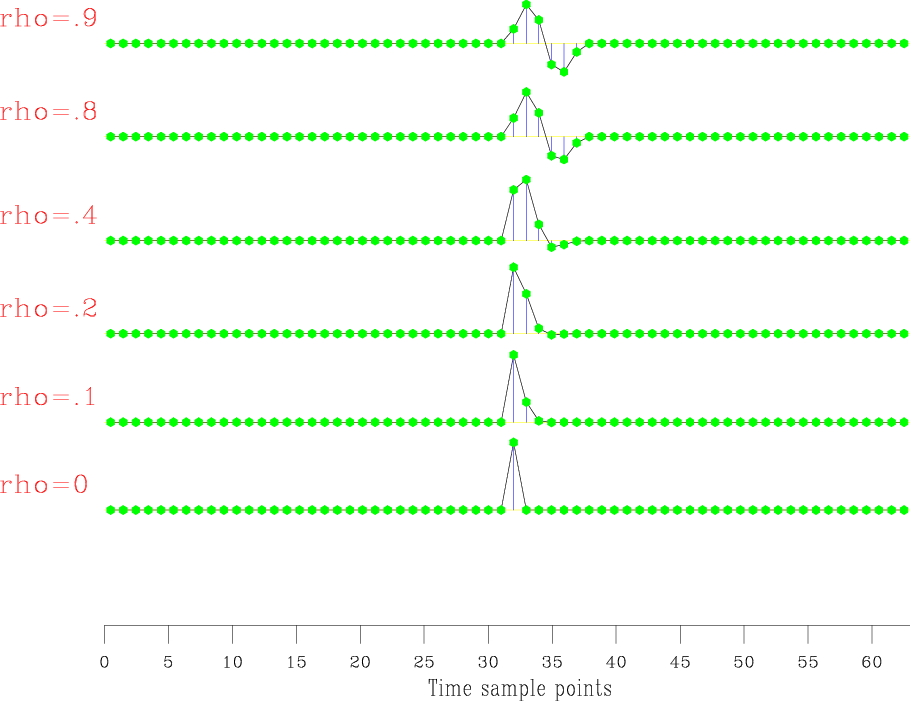
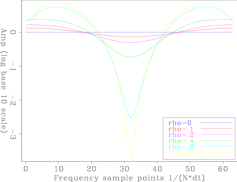
Figures 4(a) and 4(b) show the fourth-order half-Ricker wavelet in the time and frequency domains with different ![]() values.
values.
|
|---|
|
ricker-with-rho,ricker-with-rho-freq
Figure 3. The fourth-order Ricker wavelet with different |
|
|
|
|---|
|
half-ricker-with-rho,half-ricker-with-rho-freq
Figure 4. The fourth-order half-Ricker wavelet with different |
|
|
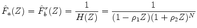
Since we have ![]() and
and
![]() in the Z domain (
in the Z domain (![]() and
and ![]() ), we have two methods to recover time-domain filter coefficients. The first one is to use
), we have two methods to recover time-domain filter coefficients. The first one is to use ![]() to get frequency domain filters and then transfer them into the time domain by an inverse Fourier transform. Another method is to use a Taylor expansion to get time-domain filter coefficients. In theory, the two methods should be the same. For less accuracy problem, we always use the frequency method in this paper.
to get frequency domain filters and then transfer them into the time domain by an inverse Fourier transform. Another method is to use a Taylor expansion to get time-domain filter coefficients. In theory, the two methods should be the same. For less accuracy problem, we always use the frequency method in this paper.
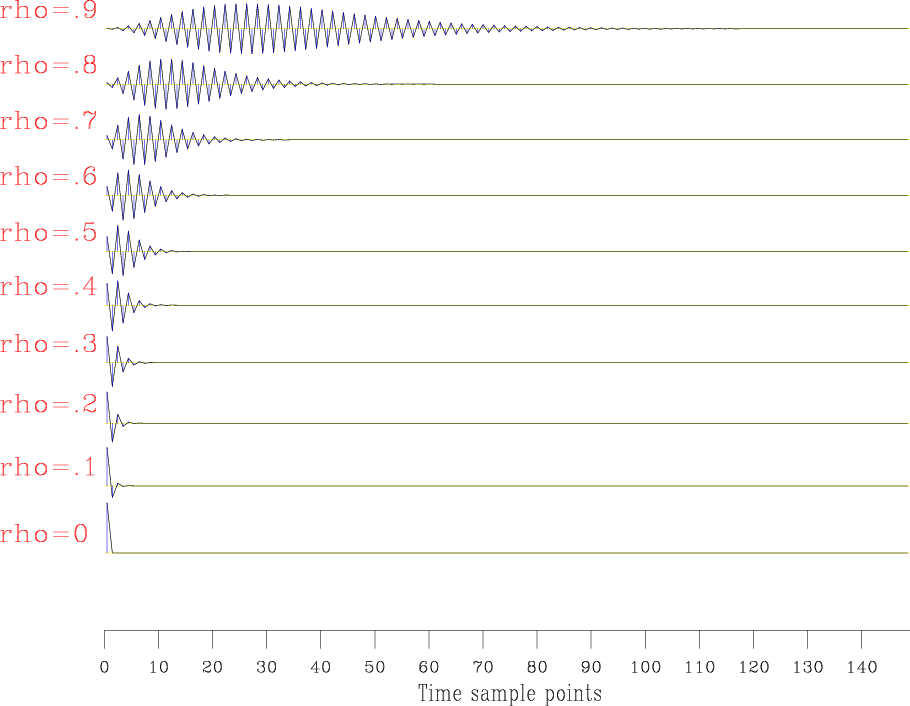
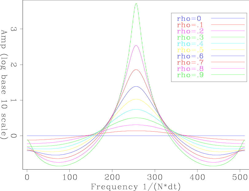
Finally we obtain the approximate inverse Ricker wavelet. Figures 5(a) and 5(b) show the inverse fourth-order causal half-Ricker wavelet (![]() ) in the time and frequency domains with different
) in the time and frequency domains with different ![]() values. The inverse anti-causal half-Ricker wavelet (
values. The inverse anti-causal half-Ricker wavelet (
![]() ) can be generated by reversing
) can be generated by reversing ![]() along the time axis.
along the time axis. ![]() and
and
![]() will be our initial guesses for bidirectional deconvolution.
will be our initial guesses for bidirectional deconvolution.
|
|---|
|
freq-domain-a,freq-domain-a-freq
Figure 5. The inverse fourth-order causal half-Ricker wavelet ( |
|
|
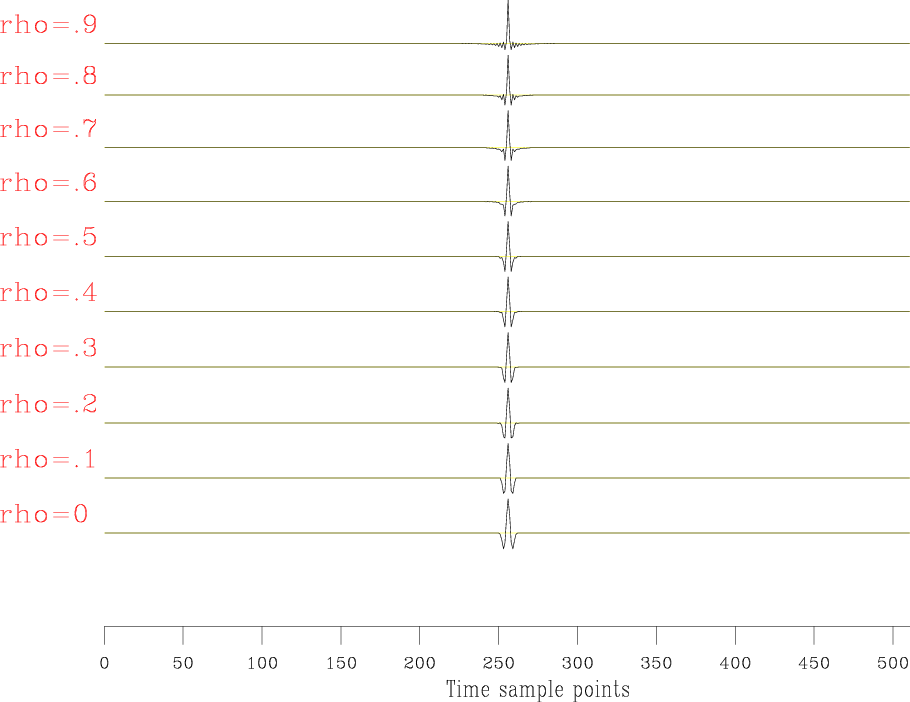
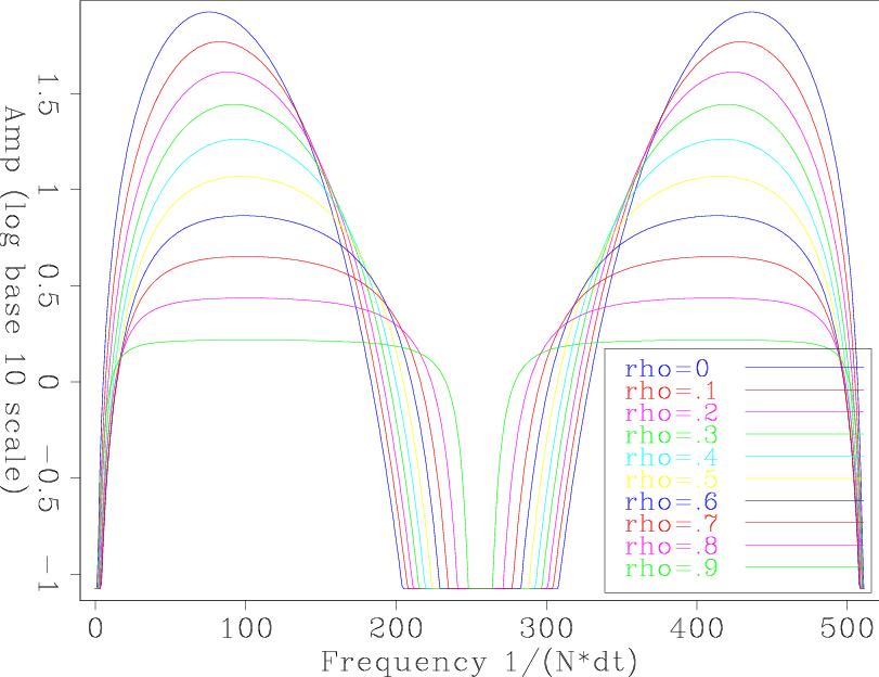
To test how good our approximation of the inverse Ricker wavelet is, we convolve our fourth-order approximate Ricker wavelet (with no ![]() factor) with our inverse Ricker wavelet (equation 12).
factor) with our inverse Ricker wavelet (equation 12).
Figures 6(a) and 6(b) show the test result in the time domain and the frequency domain with different ![]() values. We see for
values. We see for ![]() we get a good result. In particular, the frequency spectra are flatten as
we get a good result. In particular, the frequency spectra are flatten as ![]() increases.
increases.
|
|---|
|
freq-domain-result,freq-domain-result-freq
Figure 6. The test results with different |
|
|
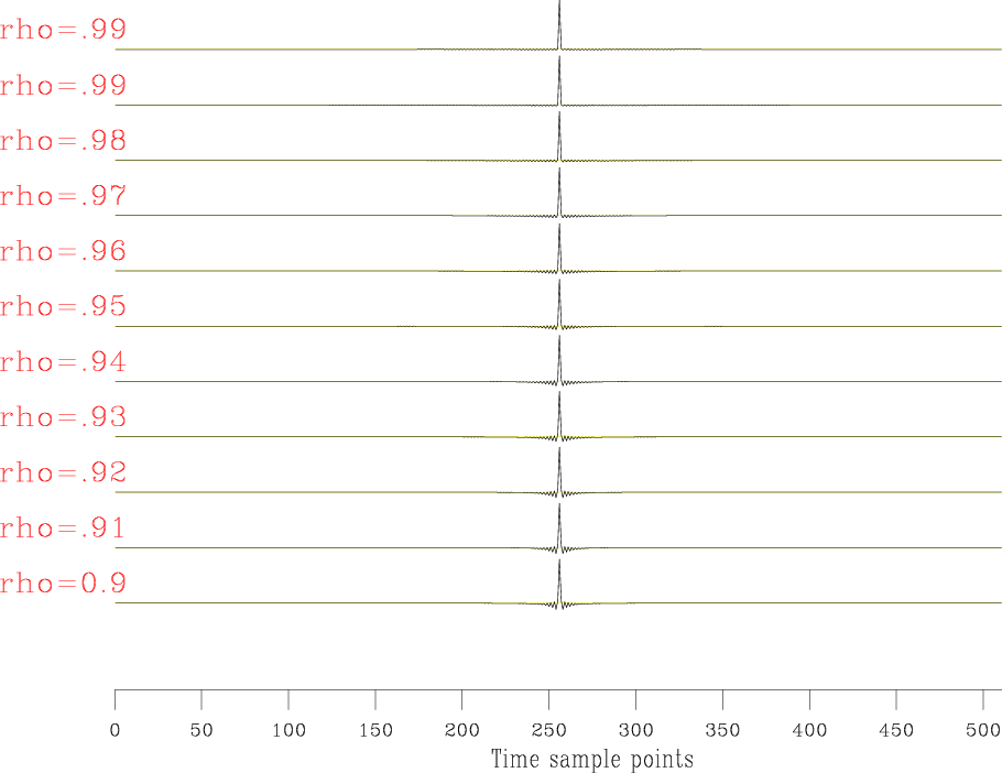
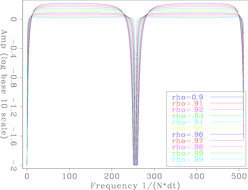
Large ![]() value can yield even better results. For large
value can yield even better results. For large ![]() , the frequency spectra are almost flat, except for two zero-value points (at 0 frequency and the Nyquist frequency). Figures 7(a) and 7(b) show these results.
, the frequency spectra are almost flat, except for two zero-value points (at 0 frequency and the Nyquist frequency). Figures 7(a) and 7(b) show these results.
|
|---|
|
freq-domain-9-99-result,freq-domain-9-99-result-freq
Figure 7. The test results with large |
|
|
However, for our goal (to use the approximate inverse Ricker wavelet as an initial guess for bidirectional deconvolution), we do not need such large ![]() values. With large
values. With large ![]() values, the filter will be long and can easily to lead to an unstable result in our deconvolution scheme.
values, the filter will be long and can easily to lead to an unstable result in our deconvolution scheme.
We now have an approximate inverse of the Ricker wavelet separated into two symmetric parts. This matches our requirements for initial guesses for filters ![]() and
and ![]() . In the next section we will test the approximation using synthetic and field data.
. In the next section we will test the approximation using synthetic and field data.
|
|
|
|
An approximation of the inverse Ricker wavelet as an initial guess for bidirectional deconvolution |