Elastic wavefield directionality vectors

Basic elastic propagation test

As a test case for the amplitude separation and displacement decomposition operators, I used a homogeneous medium, with parameters as follows:

1. P-wave velocity: $V_p = 2500 \frac{\text m}{\text s}$
2. S-wave velocity: $V_s = 1500 \frac{\text m}{\text s}$
3. Density: $\rho = 2 \frac{\text{gr}}{\text{cm}^3}$
4. Spatial sampling: $\Delta x = \Delta z = 5$$\text m$
5. Temporal sampling: $\Delta t = 0.5$   ms
6. Model dimensions: $n_x = n_z = 200$

The source function was a minimum phase Ricker wavelet, with a central frequency of $10_{hz}$ , which was applied at the center of the model. I padded the model with absorbing boundaries - an additional $16$ elements in each direction. The wavefield propagation snapshots shown below are all at propagation time $T = 250$   ms , and are shown without the surrounding absorbing boundaries.

Figure 3 is a snapshot of the propagation of the 2D elastic wavefield, at time $T = 250$   ms . In this case, the source is a pressure source, meaning that theoretically, only P-waves should be generated. The top figures show the displacements in the X direction $(U_x)$ , and in the Z direction $(U_z)$ . The bottom figures are the result of applying the Helmholtz separation to the wavefield (equation 6). The P-wave is shown on the bottom left, and has the typical appearance of an acoustic wave in a homogeneous acoustic medium. The S-wave is on the bottom right, and ideally we would see nothing there. However, the artifacts seen at the edges are the result of minute reflections off the absorbing boundaries. Since the propagation is elastic, a wave mode conversion occurs at these boundaries as a result of a very slight impedance contrast artificially produced by the absorbtion, and shear wave energy appears. This is actually a validation of the correct behaviour of the propagation code. However, as part of future work, it may be worth trying to do impedance matching along the boundaries to improve their effectiveness.

0amp-and-disp Figure 3. 2D elastic propagation snapshot at $T = 250$   ms for a pressure source. X is the vertical direction, Z is horizontal. Top left: displacements in X direction. Top right: displacements in Z direction. Bottom left: P-wave amplitude, acquired by Helmholtz separation. Bottom right: S-wave amplitude.

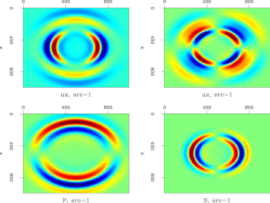
Figure 4 is similar to Figure 3, but in this case the source is a vertical dipole source, which excites both pressure and shear wave modes. These modes are apparent on the bottom row of the figure, which shows the result of applying Helmholtz separation to this wavefield. The pressure wave is radiating in the vertical direction, since the source was vertical. The shear wave is propagating in the horizontal direction, with the particle motion itself being vertical. The displacement snapshots on the top row of the figure show the $U_x$ and $U_z$ displacements, respectively. These displacements are a combination of P and S displacements in each direction. The vertical displacements $(U_x)$ are more dominant than the horizontal ones $(U_z)$ , because the source excites motion in the vertical direction.

1amp-and-disp Figure 4. 2D elastic propagation snapshot at $T = 250$   ms for a vertical dipole source. X is the vertical direction, Z is horizontal. Top left: displacements in X direction. Top right: displacements in Z direction. Bottom left: P-wave amplitude, acquired by Helmholtz separation. Bottom right: S-wave amplitude.

Elastic wavefield directionality vectors