|
|
|
|
Elastic wavefield directionality vectors |
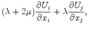
The elastic isotropic wave equation in index notation reads:
where
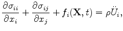 are the normal stresses,
![]() are the transverse stresses,
are the transverse stresses, ![]() is the source function in direction
is the source function in direction ![]() ,
, ![]() is the spatial source location operating at time
is the spatial source location operating at time ![]() ,
, ![]() is density and
is density and ![]() is the displacement. The stresses are propagated using the stress-displacement relation:
is the displacement. The stresses are propagated using the stress-displacement relation:
where 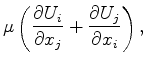 and
and ![]() are the Lame elastic constants.
are the Lame elastic constants.
The finite-difference implementation follows the staggered grid methodology of Virieux (1986). The code I am using implements the variable grid size finite difference method, developed by Wu and Harris (2002), although I have not used the grid size variability so far. The code performs 3D elastic wavefield propagation, and was ported to Fortran90 by Robert Clapp of SEP.
|
|
|
|
Elastic wavefield directionality vectors |