Elastic wavefield directionality vectors

Determination of polarization angle to the vertical

The following figures are the result of applying linear regression to the displacement fields and then calculating the polarization's angle to the vertical (equations 28 and 29), within the same time windows at which the polarization coefficient is calculated. If the polarization coefficient is below $r=0.8$ , then the angle is set to a clipped value (greater than $90^o$ ; clipped angles are red), so that the polarization coefficient figures and the angle figures display similar clipped regions. This is a visualization of the eventual methodolgy I intend to implement: when polarization cannot be estimated, I do not wish to bring the wavefield data from that location into an angle gather.

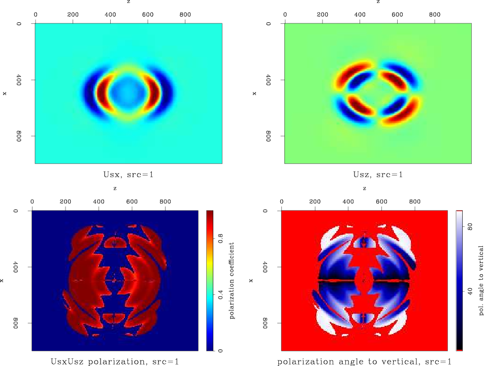
Figure 19 is a snapshot at propagation time $T = 208$ms of the undecomposed displacements (top), the polarization coefficient field (bottom-left) and the polarization angle-to-vertical field (bottom-right). There is a single pressure source at the center. The color in the angle field ranges from white to black, where black designates vertical polarization $(\theta = 0^o)$ , and white designates horizontal polarization $\theta = 90^o)$ . In this figure, because there is only a single P-wave, the field is highly linearly polarized. Also, the polarization direction is the propagation direction. The angle field therefore is a good indication of the propagation direction, and this can be verified when observing the displacement fields. However, notice the ``waviness'' along the diagonals radiating from the center of the field, where the source is located. If the polarization estimation were perfect, we would expect all lines radiating from the source to have the same color, meaning the same polarization angle.

0U-disp-and-ang Figure 19. Displacement snapshot at $T = 208$   ms for a pressure source. Top: displacements in X and Z directions. Bottom left: polarization coefficient clipped below $r=0.8$ . Bottom right: angle of polarization direction to the vertical (Dark blue= $0^o$ , white= $90^o$ ).

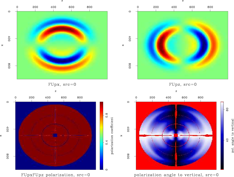
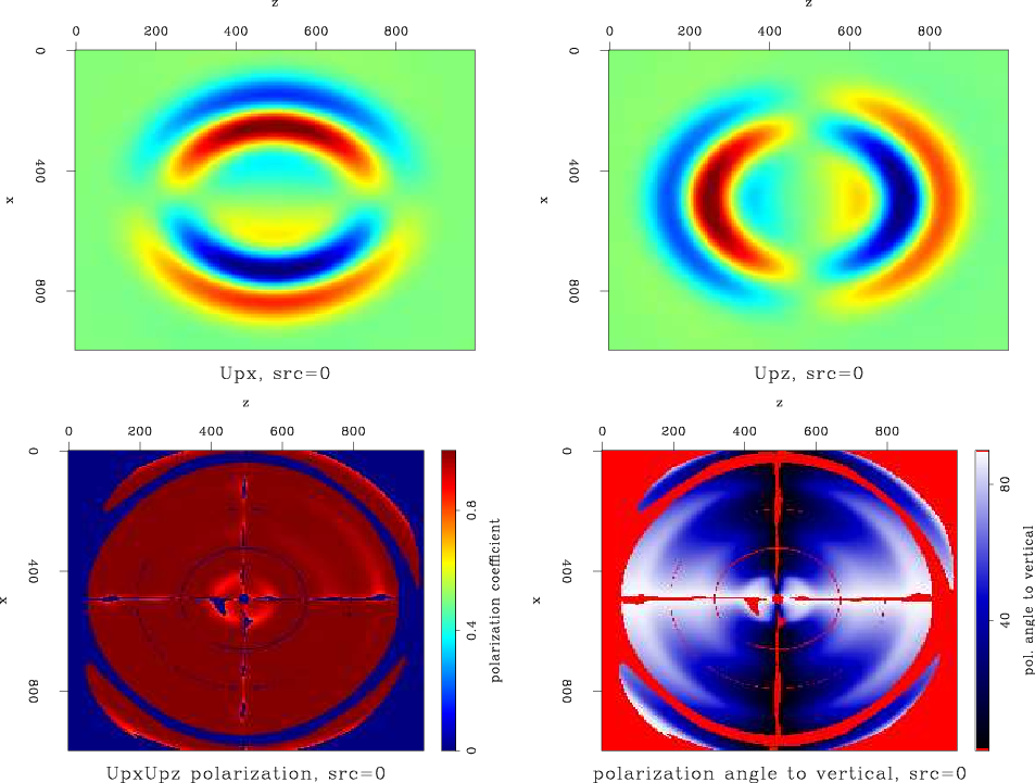
Figures 20 and 21 are the result of wavenumber domain decomposition and space domain decomposition, respectively. As the decomposition should, theoretically, have no effect on this single mode wavefield, we expect these figures to be identical to Figure 19. The polarization coefficient and the polarization angle panels in Figure 20 are very similar to their undecomposed counterparts, but in Figure 21 a circular artifact is evident. I attribute this artifact to the helical deconvolution by which the decomposition was done (equation 24). As a result of the length of the filter, data is ``spread'' from one part of the model to another, in this case from the surrounding absorbing boundary region to the internal part of the wavefield. As the filter length changes, the amplitude and location of this artifact changes. If the filter is too long, data from the bottom edge of the wavefield could actually be incorporated into the top edge, due to the wrap-around of the helical coordinate system.

0FUp-disp-and-ang Figure 20. P wave displacement snapshot at $T = 208$   ms for a pressure source, decomposition in wavenumber domain. Top: displacements in X and Z directions. Bottom left: polarization coefficient clipped below $r=0.8$ . Bottom right: angle of polarization direction to the vertical (Dark blue= $0^o$ , white= $90^o$ ).

0Up-disp-and-ang Figure 21. P wave displacement snapshot at $T = 208$   ms for a pressure source, decomposition in space domain. Top: displacements in X and Z directions. Bottom left: polarization coefficient clipped below $r=0.8$ . Bottom right: angle of polarization direction to the vertical (Dark blue= $0^o$ , white= $90^o$ ).

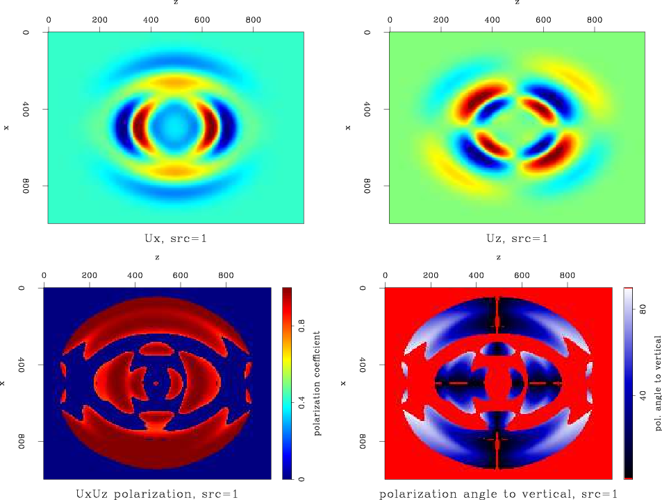
Figure 22 is the undecomposed displacements snapshot at propagation time $T = 208$ms , for a vertical dipole source at the center of the field. This excites both P and S wave modes, and therefore the displacements are a mixture of P and S. This is the reason for the smaller region of linear polarization seen in the bottom-left of the figure, in comparison to Figure 19. The bottom-right of the figure shows the polarization's angle to vertical. A dark region, indicating vertical polarization, is visible along both directions away from the source. The vertical polarization to the right and left of the source are a result of vertical S displacements, and those that are over and under the source are a result of vertical P displacements.

1U-disp-and-ang Figure 22. Displacement snapshot at $T = 208$   ms for a vertical dipole source. Top: displacements in X and Z directions. Bottom left: polarization coefficient clipped below $r=0.8$ . Bottom right: angle of polarization direction to the vertical (Dark blue= $0^o$ , white= $90^o$ ).

Figures 23 and 24 are the decomposed P displacements of the dipole-source generated field, by wavenumber and by space domain decomposition, respectively. They both exhibit the generally correct behaviour for the P-wave - it propagates mostly vertically, and the polarization direction should be likewise mostly vertical, radiating vertically from the source at the center (refer to Figure 4). However, the smoothness of the polarization coefficient field derived by space domain decomposition is much greater than the one derived by wavenumber domain decomposition. This in turn affects the smoothness of the polarization angle field.

1FUp-disp-and-ang Figure 23. P wave displacement snapshot at $T = 208$   ms for a vertical dipole source, decomposition in wavenumber domain. Top: displacements in X and Z directions. Bottom left: polarization coefficient clipped below $r=0.8$ . Bottom right: angle of polarization direction to the vertical (Dark blue= $0^o$ , white= $90^o$ ).

1Up-disp-and-ang Figure 24. P wave displacement snapshot at $T = 208$   ms for a vertical dipole source, decomposition in space domain. Top: displacements in X and Z directions. Bottom left: polarization coefficient. Bottom right: angle of polarization direction to the vertical (Dark blue= $0^o$ , white= $90^o$ ).

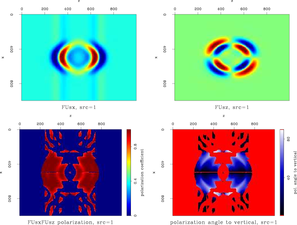
Figures 25 and 26 are the decomposed S displacements of the dipole-source generated field, by wavenumber and by space domain decomposition, respectively. In this case, we expect there to be a mostly vertically polarized wave, propagating to the sides away from the source at the center. This effect can be seen in both figures, on the bottom-right panel. Just as was shown above for the P-wave, the relative smoothness of the space domain decomposition compared to the wavenumber domain decomposition is evident.

1FUs-disp-and-ang Figure 25. S wave displacement snapshot at $T = 208$   ms for a vertical dipole source, decomposition in wavenumber domain. Top: displacements in X and Z directions. Bottom left: polarization coefficient clipped below $r=0.8$ . Bottom right: angle of polarization direction to the vertical (Dark blue= $0^o$ , white= $90^o$ ).

1Us-disp-and-ang Figure 26. S wave displacement snapshot at $T = 208$   ms for a vertical dipole source, decomposition in space domain. Top: displacements in X and Z directions. Bottom left: polarization coefficient clipped below $r=0.8$ . Bottom right: angle of polarization direction to the vertical (Dark blue= $0^o$ , white= $90^o$ ).

Elastic wavefield directionality vectors