Reverse-time migration using wavefield decomposition

Origin of RTM artifacts due to backscattered waves

In order to investigate the origin of RTM artifacts due to backscattered waves, let us assume a flat interface with high velocity contrast as shown in Figure 7. The source wavefield (solid) and receiver wavefield (dashed) are extrapolated using a full propagator corresponding to Equation 2. When the propagated wavefields encounter this strong interface, part of the energy is transmitted and carries on downwards, while the remaining energy is reflected back to the surface. This phenomenon is observable for both source and receiver wavefields. Thus, at any point above the reflector, the corresponding source and receiver wavefields have exactly the same propagation paths, along which non-zero cross-correlations are produced (Liu et al., 2011; Robein, 2010). Accordingly, the cross-correlation of these wavefields creates not only the reflectivity image but also noise at all nonreflecting points along the propagation paths, such as point B and point C in Figure 7. Thus, low-frequency noise is a common characteristic of the RTM image with a strong reflector.

rtm-artifact1,rtm-artifact2
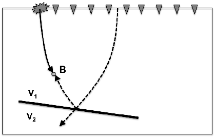
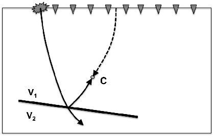
Figure 7. The solid lines represent the propagation paths of a source wavefield, where the arrows indicate the propagation direction with time running forward. The dashed lines represent the propagation paths of a receiver wavefield, where the arrows indicate the propagation direction with time running backwards.

Note that, in this paper, I use the terms with the suffix -going such as upgoing and downgoing for describing the propagation direction of wavefields with time running forward. At point B in Figure 7(a), the downgoing source wavefield coincides in time with the propagated receiver wavefield that has been reflected. This receiver wavefield is indeed propagating downward with time running forward, i.e. downgoing receiver wavefield. On the other hand, at point C in Figure 7(b), the upgoing reflected source wavefield coincides in time with the upgoing receiver wavefield.

At either point B or point C in Figure 7, both source and receiver wavefields are propagating in the same direction and the same path with time running forward. Thus, the correlation-based images at point B and point C are caused by forward scattering events. These images are undesirable and can be considered to be noise, because they do not represent a reflected event. In contrast, at any point on the reflector, source and receiver wavefields are propagating in opposite directions with respect to the normal vector of the reflector. Thus, the cross-correlation of these source and receiver wavefields, which results from backward scattering events, produces the desired image.

To keep only energy corresponding to backward scattering events in the final image, we might apply the cross-correlation to only the source and receiver wavefields that are propagating in opposite directions with respect to the reflector normal. This approach requires us to compute the propagation direction of both the source and receiver wavefields at every point in the computational domain. Although this approach involves intensive computation, it can provide the reflectivity images without forward scattering noise.

The computation of the wavefield propagation direction at every point in the compuational domain can be done using a Poynting vector (Yoon et al., 2004). This works well for simple models, but it does not produce satisfactory results in complex subsurface structures (Guitton et al., 2006). Xie and Wu (2006) applied the local one-way propagator, which is endowed with the Rayleigh integral, in order to decompose the wavefields. Another practical method is to decompose the wavefields in the Fourier domain in order to obtain the appropriate directional components of the wavefields based on Cartesian directions (Liu et al., 2007). This method is robust and worth investigation.

Wavefield decomposition based on Cartesian propagation directions can be used to modify the RTM imaging condition. This application was introduced by Liu et al. (2007,2011), Suh and Cai (2009), and Fei et al. (2010). They all introduced methods to decompose source and receiver wavefields into one-way components along horizontal directions (leftgoing/rightgoing) and vertical directions (upgoing/downgoing). They then applied the zero-lag cross-correlation as the imaging condition to the appropriate combinations of these wavefield components. The results showed that such a method can effectively eliminate unwanted artifacts from conventional RTM images, and image quality was also improved.

Liu et al. (2007) applied wavefield decomposition in the F-K domain and obtained promising RTM results. The same authors later showed that a cheaper wavefield decomposition method in the wavenumber domain (T-K domain) can also provide the same results (Liu et al., 2011). Moreover, Suh and Cai (2009) applied a fan filter in the T-K domain before decomposing the filtered wavefields in the F-K domain. This approach produces better RTM images, but the computational cost significantly increases. In addition, Fei et al. (2010) illustrated how the decomposition method attenuates the artifacts in RTM images. However, Fei et al. (2010) did not provide the detail of the method they used to decompose the wavefields.

As mentioned above, Liu et al. (2007,2011) advocated using wavefield decomposition for RTM in the Fourier domain. Next section, I describe this method with both horizontal and vertical propagation decompositions.

Reverse-time migration using wavefield decomposition