|
|
|
|
Anisotropic tomography with rock physics constraints |
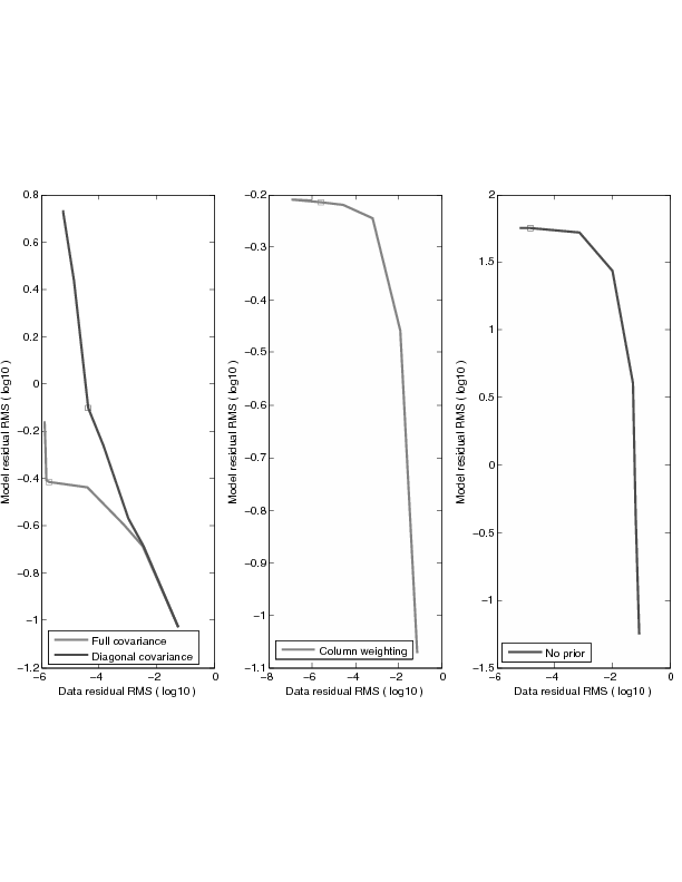
 in equation 7 and investigate the posterior distribution of the inversion (Hansen and O'Leary, 1993). Typical L-curve has two distinct parts: one vertical part where the solution is dominated by the data fitting and one horizontal part where the solution is dominated by the model styling. The corner of the L-curve corresponds to a good balance between minimization of both fitting goals. In Figure 5, we obtain the L-curve for each inversion scheme for the shale (sandy shale) model in log-log scale by varying
from
will place the solution right at the corner of the L-curve, as in the case of using the full covariance. The "7-curve" shape in the log-log scale (which is still an "L-curve" in absolute scale) shows a relatively poor estimation of the covariance matrix, hence indicating difficulties in finding a proper damping parameter
.
in equation 7 and investigate the posterior distribution of the inversion (Hansen and O'Leary, 1993). Typical L-curve has two distinct parts: one vertical part where the solution is dominated by the data fitting and one horizontal part where the solution is dominated by the model styling. The corner of the L-curve corresponds to a good balance between minimization of both fitting goals. In Figure 5, we obtain the L-curve for each inversion scheme for the shale (sandy shale) model in log-log scale by varying
from
will place the solution right at the corner of the L-curve, as in the case of using the full covariance. The "7-curve" shape in the log-log scale (which is still an "L-curve" in absolute scale) shows a relatively poor estimation of the covariance matrix, hence indicating difficulties in finding a proper damping parameter
.
Finally, to move beyond the deterministic inversion which produces only one solution, we perform the null-space analysis following the work flow proposed by Osypov et al. (2008). The effective null-space of an operator can be sampled by an iterative Lanczos eigen-decomposition method. The right panel on Figure 1 shows the null-space projection (darker dots) overlaid on the approximate prior distribution (smaller dots) when the full covariance scheme is used. It is obvious that the full covariance matrix representation produces a good estimation to the true prior (by the similarity of the cloud shape on the left panel and the right panel). Also, the null-space projection suggests that higher uncertainty in anisotropic parameters for higher velocities, which often means greater depth, is embedded in rock physics knowledge. The reduced volume of the cloud shows the value of information that the data bring into the inversion.
|
|---|
|
L-curve
Figure 5. L-curve for the shale (sandy shale) model inversion. |
|
|
|
|
|
|
Anisotropic tomography with rock physics constraints |