|
|
|
|
Anisotropic tomography with rock physics constraints |
In practice, we usually formulate the seismic tomography problem as an inversion problem with another model space regularization term. Then the objective function reads:
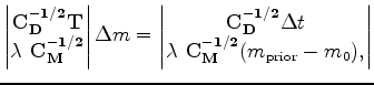
We can also obtain the normal equation representation of the objective function by taking the derivative of equation 5 with respect to ![]() :
:
 is the balancing factor between the data fitting equation and the model fitting equation. For the synthetic study here, we may assume
To speed up the convergence, we turn this regularized problem into a preconditioned problem by doing a variable substitution:
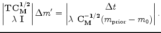 , and the real model updates are obtained by
For a multi-parameter model inversion, we assume the model covariance can be fully decoupled into two different parts: spatial covariance for each parameter, and the local cross-parameter covariance. Mathematically, that translates into:
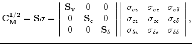 is a spatial smoothing matrix, and
can be estimated according to the user's assumption for the smoothness of different parameters. For example, the steering filters (Clapp et al., 2004; Fomel, 1994) provide a good choice to incorporate the structural information of the subsurface. The local cross-parameter covariance can be estimated from the rock physics modeling (Bachrach, 2010a).
is a spatial smoothing matrix, and
can be estimated according to the user's assumption for the smoothness of different parameters. For example, the steering filters (Clapp et al., 2004; Fomel, 1994) provide a good choice to incorporate the structural information of the subsurface. The local cross-parameter covariance can be estimated from the rock physics modeling (Bachrach, 2010a).
|
|---|
|
covariance
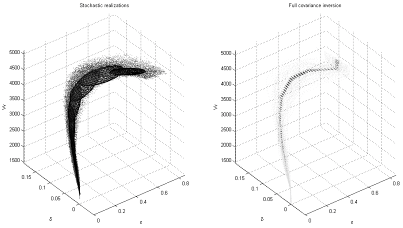
Figure 1. Left: Stochastic realizations of a rock physics modeling for shale and sandy shale. The ellipsoids are fitted locally to describe the multi-Gaussian relationship among the parameters. Right: Small dots in the background are the estimated prior distribution by the operator using the ellipsoids on the left. Larger dots are the null-space projection of the operator. |
|
|
The left panel on Figure 1 shows an example of the stochastic realizations of a rock physics model for shale and sandy shale. The dots are scattered ![]() ,
, ![]() and
and ![]() results of hundreds of realizations, while the nine ellipsoids are fitted locally with
results of hundreds of realizations, while the nine ellipsoids are fitted locally with ![]() the controlling variable to describe the multi-Gaussian relationship among the parameters. With a statistical study of the laboratory measurements on the cores, the range of the required input parameters for the rock physics model has been limited to a relatively narrow range, which leads to tight ellipsoids in Figure 1. We refer interested readers to details in Bachrach (2010a).
the controlling variable to describe the multi-Gaussian relationship among the parameters. With a statistical study of the laboratory measurements on the cores, the range of the required input parameters for the rock physics model has been limited to a relatively narrow range, which leads to tight ellipsoids in Figure 1. We refer interested readers to details in Bachrach (2010a).
In this paper, we build the cross-parameter covariance matrix for each grid point in the subsurface according to the velocity, and linearly interpolate between the ellipsoids to which the velocity value belongs. Notice that additional non-linearity has been introduced during this process. Better methods to utilize the stochastic realizations could fit ellipsoids centered at every velocity value, which can be more precise but outside the scope of this study.
|
|
|
|
Anisotropic tomography with rock physics constraints |