Correlation-based wave-equation migration velocity analysis

Synthetic Examples

The background model has a constant velocity of 2500 m/s. The model is 4000 m wide and 2800 m deep. The spatial sampling is 20 m, and the temporal sampling is 3 ms. A Ricker wavelet with a fundamental frequency of 15 Hz is used to model the data. The receiver spacing is 20 m, and the shot spacing is 80 m. The reflector is at a depth of 2200 m. Born modeling was used in both the observed and the calculated data. There are three anomalies that I will estimate: first, a negative Gaussian anomaly at a depth of 1300 m with a maximum velocity of 800 m/s, second, a constant velocity decrease of 250 m/s, and third, a constant velocity increase of 250 m/s. First, I will compute the optimum WEMVA gradient by applying the forward and adjoint of these slowness perturbations. The results are shown in figures 1(a), 1(c) and 1(e). Then, I compute the angle-domain common-image gathers using the background velocity of the data with the three anomalies, which are shown in figures 1(b), 1(d) and 1(f).

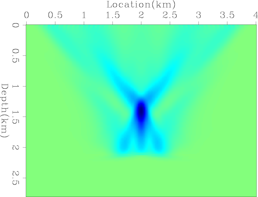
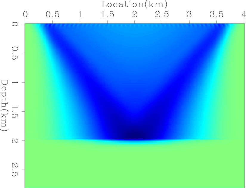
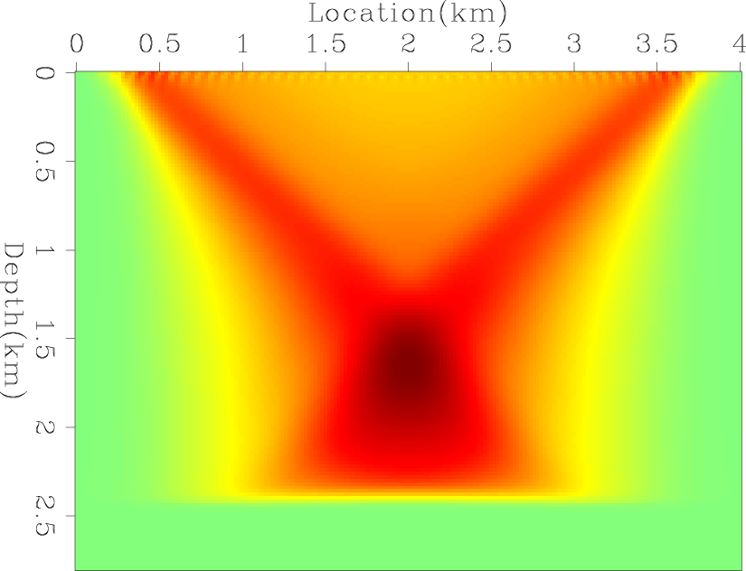
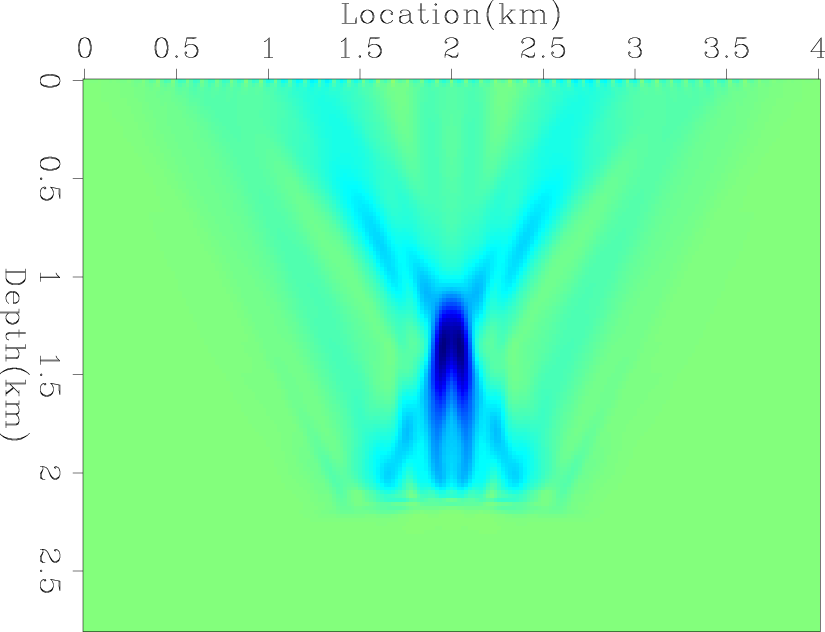
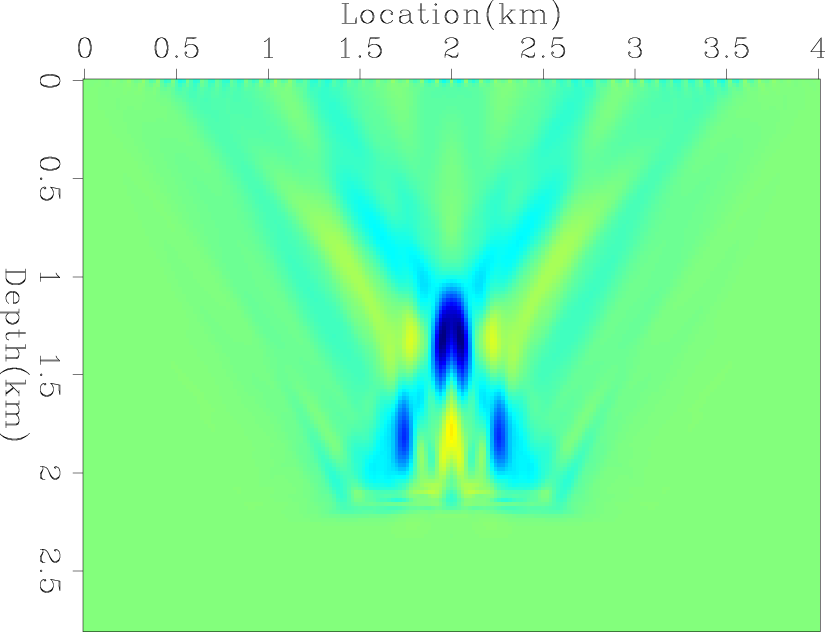
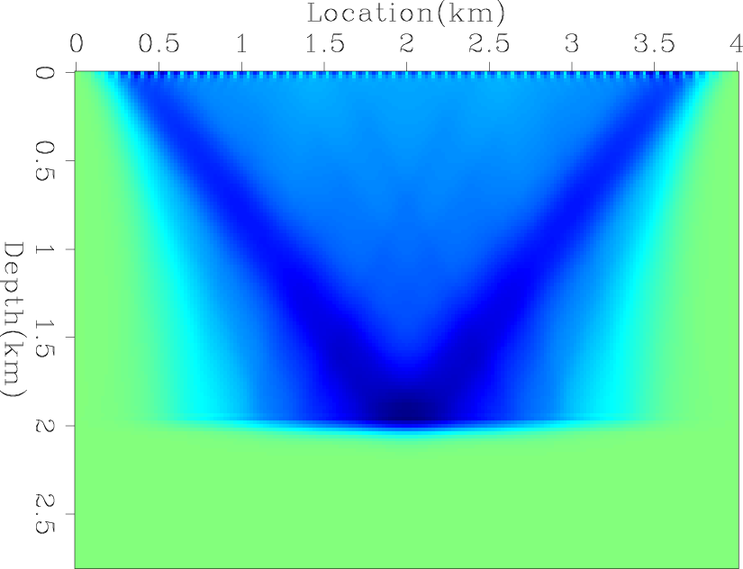
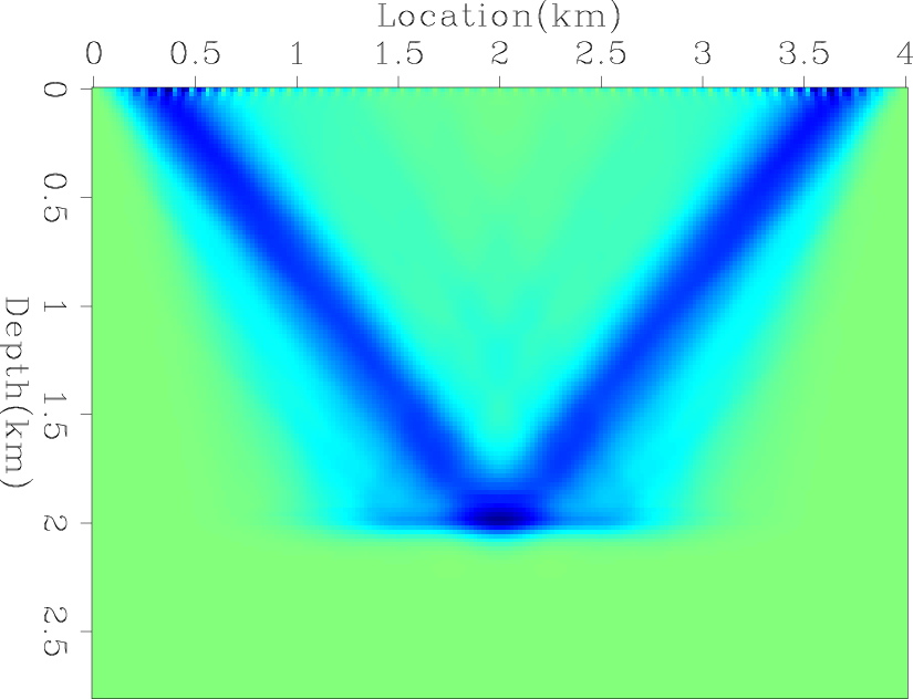
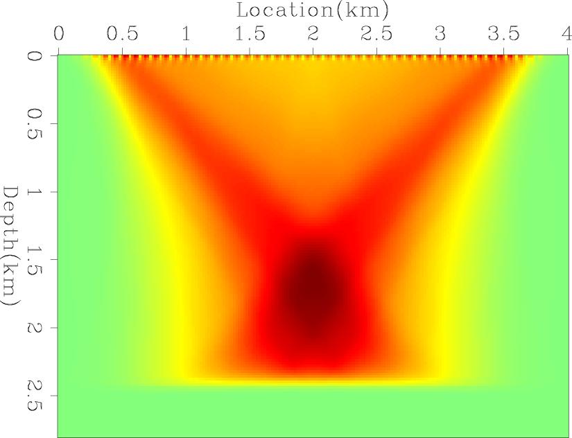
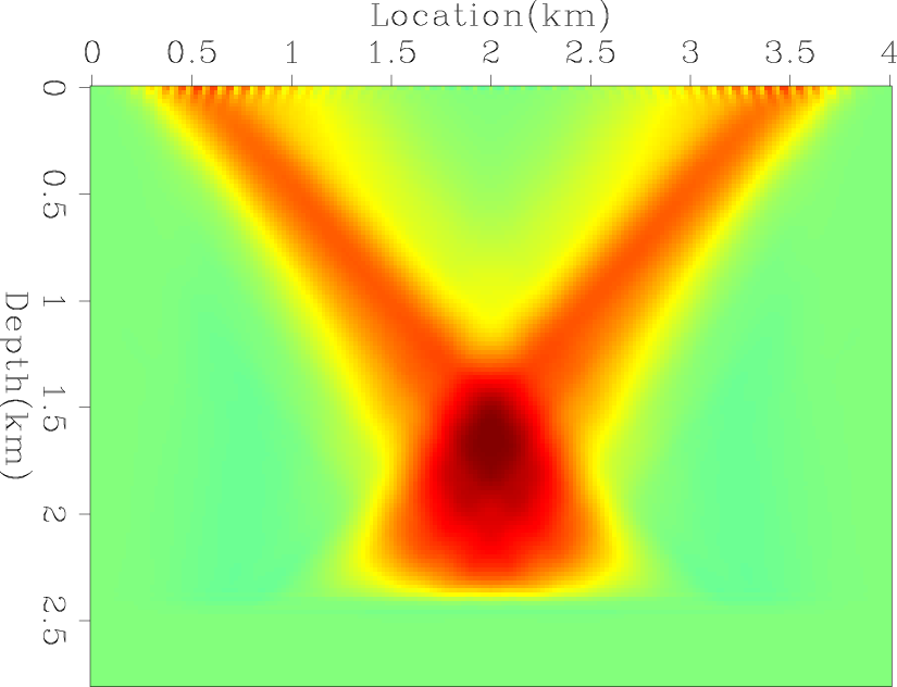
Next I show the results of applying the first term of the tomographic operator in equation (10). First, I use the true reflector depth to create the reference image and use it in our method to generate the gradients for the three anomalies, as shown in figures 2(a), 2(c) and 2(e). Finally, I use the apparent reflector depth, i.e. the depth extracted from the zero-subsurface-offset image, to create the reference image and generate the gradients shown in figures 2(b), 2(d) and 2(f). The correlation lags were picked automatically by choosing the maximum value of the cross-correlation function.

dS1,adcig1,dS2,adcig2,dS3,adcig3
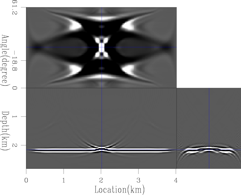
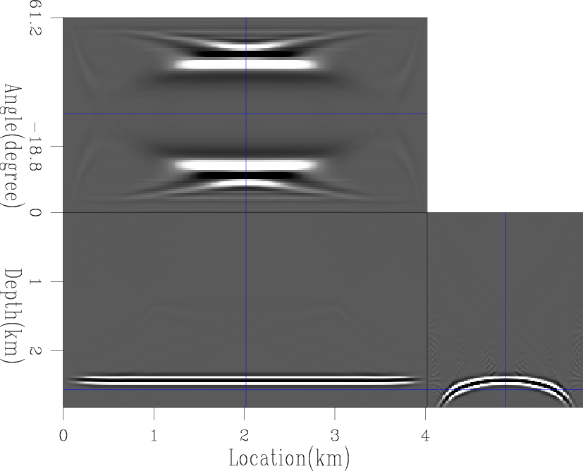
Figure 1. The left column shows the optimum WEMVA gradient of (a) a negative Gaussian anomaly, (c) a negative bulk shift and (e) a positive bulk shift. The right column shows the corresponding ADCIGs.

dS221,dS321,dS222,dS322,dS223,dS323
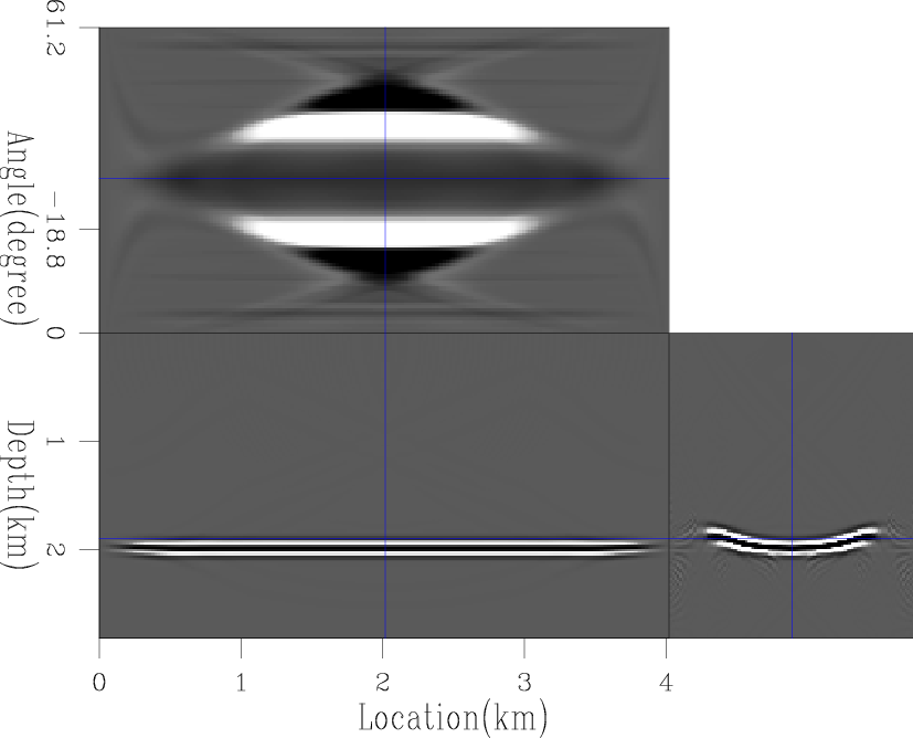
Figure 2. The left column shows the correlation-based WEMVA gradients using the true depth for the reference image. The right column shows the correlation-based WEMVA gradients using the apparent depth for the reference image.

Correlation-based wave-equation migration velocity analysis