Model-building with image segmentation and fast image updates

Image updates

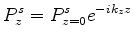
Image updates and comparisons will be performed using shot-profile migration (see Biondi (2005)). In general, this type of migration uses downward-continued source ($P^s$ ) and receiver ($P^g$ ) wavefields:

$$P_z^s=P_{z=0}^se^{-ik_zz}$$ (1)

$$P_z^g=P_{z=0}^ge^{ik_zz},$$ (2)

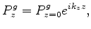where $z$ is the depth and $k_z$ is the vertical wavenumber calculated in a split-step fashion (Stoffa et al., 1990) for a given frequency $\omega$ according to

$$k_z=\sqrt{\frac{\omega^2}{v_{\mathrm{ref}}^2} - \vert\mathbf{k}\vert^2} + \left(\frac{\omega}{v(z,x)}-\frac{\omega}{v_{\mathrm{ref}}}\right),$$ (3)

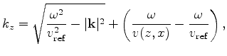where $\mathbf{k}$ is a vector containing the horizontal wavenumbers. Here, $v_{\mathrm{ref}}$ is a reference velocity that is constant at each depth step, while $v(z,x)$ is the actual estimated velocity. An image is formed by correlating the two wavefields:

$$I(z,x)=\sum_i \sum_{\omega}P_z^g(\omega,x;\mathbf{s}_i) \overline{P_z^s(\omega,x;\mathbf{s}_i)}.$$ (4)

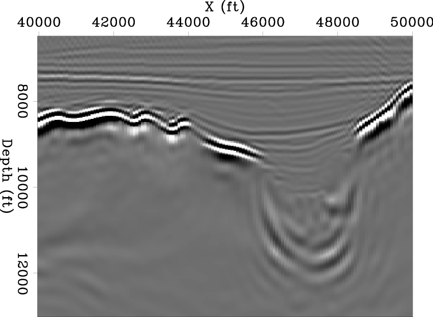
Performing full migrations is impractical for our stated purpose of allowing interpreters to quickly judge the relative accuracy of two or more possible velocity models. One way to speed up the process is to re-datum the wavefields to a depth just above the region of interest - in this case, just above the salt canyon near 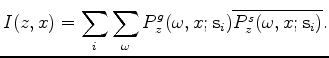$z=7500$ . If we only wish to investigate changes in a specific area of the image, we can downward continue both wavefields to this level, and inject areal source and receiver gathers. This allows us to obtain comparison images like those in Figure 5(a) and 5(b), at a computational cost an order of magnitude less than performing full migrations like the one in Figure 1(a). In this case, it is clear that the salt canyon flanks in Figure 5(a) are more sharply focused, so the salt interpretation and velocity model in Figures 3(a) and 4(a), respectively, are more accurate.

shortimg1,shortimg2
Figure 5. Images resulting from the velocity models in Figures 4(a) and 4(b). The salt canyon walls are more focused in (a), indicating the the salt interpretation in Figure 3(a) is more accurate.

Model-building with image segmentation and fast image updates